

Why CORe50?
One of the greatest goals of AI is building an artificial continual learning agent which can construct a sophisticated understanding of the external world from its own experience through the adaptive, goal-oriented and incremental development of ever more complex skills and knowledge.Yet, Continual/Lifelong learning (CL) of high-dimensional data streams is a challenging research problem far from being solved. In fact, fully retraining models each time new data becomes available is infeasible, due to computational and storage issues, while naïve continual learning strategies have been shown to suffer from catastrophic forgetting. Moreover, even in the context of real-world object recognition applications (e.g. robotics), where continual learning is crucial, very few datasets and benchmarks are available to evaluate and compare emerging techniques.
In this page we provide a new dataset and benchmark CORe50, specifically designed for assessing Continual Learning techniques in an Object Recognition context, along with a few baseline approaches for three different continual learning scenarios. Futhermore, we recently extended CORe50 to support object detection and segmentation. If you plan to use this dataset or other resources you'll find in this page, please cite the related papers:

Table of Content
1. Dataset
2. Benchmark
2.1 Differences with other common CL Benchmarks
3. Download
3.1 Dataset
3.2 Object Detection
3.3 Object Segmentation
3.4 Configuration Files
3.5 Results
3.6 Code and Data Loaders
4. Contacts
Dataset
CORe50, specifically designed for (C)ontinual (O)bject (Re)cognition, is a collection of 50 domestic objects belonging to 10 categories: plug adapters, mobile phones, scissors, light bulbs, cans, glasses, balls, markers, cups and remote controls. Classification can be performed at object level (50 classes) or at category level (10 classes). The first task (the default one) is much more challenging because objects of the same category are very difficult to be distinguished under certain poses.
The dataset has been collected in 11 distinct sessions (8 indoor and 3 outdoor) characterized by different backgrounds and lighting. For each session and for each object, a 15 seconds video (at 20 fps) has been recorded with a Kinect 2.0 sensor delivering 300 RGB-D frames.
Objects are hand hold by the operator and the camera point-of-view is that of the operator eyes. The operator is required to extend his arm and smoothly move/rotate the object in front of the camera. A subjective point-of-view with objects at grab-distance is well-suited for a number of robotic applications. The grabbing hand (left or right) changes throughout the sessions and relevant object occlusions are often produced by the hand itself.
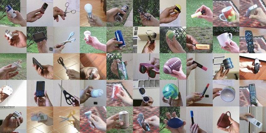
Fig.1 Example images of the 50 objects in CORe50. Each column denotes one of the 10 categories.
The presence of temporal coherent sessions (i.e., videos where the objects gently move in front of the camera) is another key feature since temporal smoothness can be used to simplify object detection, improve classification accuracy and to address semi-supervised (or unsupervised) scenarios.
In Fig. 1 you can see some image examples of the 50 objects in CORe50 where each column denotes one of the 10 categories and each row a different object. The full dataset consists of 164,866 128×128 RGB-D images: 11 sessions × 50 objects × (around 300) frames per session. Three of the eleven sessions (#3, #7 and #10) have been selected for test and the remaining 8 sessions are used for training. We tried to balance as much as possible the difficulty of training and test session with respect to: indoor/outdoor, holding hand (left or right) and complexity of the background. For more information about the dataset take a look a the section "CORe50" in the paper.
Benchmark
Popular datasets such as ImageNet and Pascal VOC, provide a very good playground for classification and detection approaches. However, they have been designed with “static” evaluation protocols in mind; the entire dataset is split in just two parts: a training set is used for (one-shot) learning and a separate test set is used for accuracy evaluation.Splitting the training set into a number of batches is essential to train and test continual learning approaches, a hot research topic that is currently receiving much attention. Unfortunately, most of the existing datasets are not well suited to this purpose because they lack a fundamental ingredient: the presence of multiple (unconstrained) views of the same objects taken in different sessions (varying background, lighting, pose, occlusions, etc.). Focusing on Object Recognition we consider three continual learning scenarios:
- New Instances (NI): new training patterns of the same classes becomes available in subsequent batches with new poses and environment conditions (illuminations, background, occlusions, etc..). A good model is expected to incrementally consolidate its knowledge about the known classes without compromising what it learned before.
- New Classes (NC): new training patterns belonging to different classes becomes available in subsequent batches. In this case the model should be able to deal with the new classes without losing accuracy on the previous ones.
- New Instances and Classes (NIC): new training patterns belonging both to known and new classes becomes available in subsequent training batches. A good model is expected to consolidate its knowledge about the known classes and to learn the new ones.


Fig. 2 Mid-CaffeNet accuracy in the NI, NC and NIC scenarios (average over 10 runs).
As argued by many researchers, naïve approaches cannot avoid catastrophic forgetting in complex real-world scenarios such as NC and NIC. In our work we have designed simple baselines which can perform markedly better than naïve strategies but still leave much room for improvements (see Fig. 2). Check it out the full results on our paper or download them as tsv or python dicts in the section below!
Differences with other common CL Benchmarks
As you probably noted from the description above, our benchmark is somehow different from the common benchmarks used in the continual Learning literature where the focus is mostly about learning a (short) sequence of tasks:
If you want to learn more about this distinction you can visit our "Continual Learning Benchmarks" web page where we keep track of all the most common benchmarks in CL and the main differences among them (We also keep track of the most popular "Continual Learning Strategies" and on which benchmark they have been assessed here).Please also note that we decided for simplicity to keep the test set fixed across all batches (check section 5.2 of the paper for further discussions about this choice).
Download
In order to facilitate the usage of the benchmark we freely release the dataset, the code to reproduce the baselines and all the materials which could be useful for speeding-up the creation of new continual learning strategies on CORe50.Dataset
The dataset directory tree is not that different from what you may expect. For each session (s1, s2, ..., s11) we have 50 directories (o1, o2, ..., o50) representing the 50 objects contained in the dataset. Below you can see to which class each object instance id corresponds to:
[o1, ..., o5] -> plug adapters
[o6, ..., o10] -> mobile phones
[o11, ..., o15] -> scissors
[o16, ..., o20] -> light bulbs
[o21, ..., o25] -> cans
[o26, ..., o30] -> glasses
[o31, ..., o35] -> balls
[o36, ..., o40] -> markers
[o41, ..., o45] -> cups
[o46, ..., o50] -> remote controls
In each object directories, the temporal coherent frames are characterized by an unique filename with the format "C_[session_num]_[obj_num]_[frame_seq_id].png" :
CORe50/
  |
  |--- s1/
  |    |------ o1/
  |    |       |---- C_01_01_XXX.png
  |    |       |---- ...
  |    |
  |    |------ o2/
  |    |------ ...
  |    |------ o50/
  |
  |--- s2/
  |--- s3/
  |--- ...
  |--- s11/
Since we make available both the 350 x 350 original images and their cropped version (128 x 128), we thought it would be useful also to release the bounding boxes with respect to the original image size.
The bbox coordinates for each image are automatically extracted based on a very simple tracking technique, briefly described in the paper. In the bbox.zip you can download below you will find for each object and session a different txt file. Each file follows the format:
Color000: 142 160 269 287
Color001: 143 160 270 287
Color002: 145 160 272 287
Color003: 149 160 276 287
Color004: 149 159 276 286
...
So, for each image ColorID, we have the bbox in the common format [min x, min y, max x, max y] of the image coordinates system.
If you are a Python user you can also benefit by our npz version of the dataset core50_imgs.npz accompanied by the paths.pkl file which contains the path corresponding to each image.
 # loading the npz and picked file
 >>> import numpy as np
 >>> import pickle as pkl
 >>> pkl_file = open('paths.pkl', 'rb')
 >>> paths = pkl.load(pkl_file)
 >>> imgs = np.load('core50_imgs.npz')['x']

 # Files dimensions
 >>> print imgs.shape
 (164866, 128, 128, 3)
 >>> print len(paths)
 164866
In order to better track the moving objects or to further improve the object recognition accuracy, we release also the depth map in the same format we have seen before for the colored images:
CORe50/
  |
  |--- s1/
  |    |------ o1/
  |    |       |---- D_01_01_XXX.png
  |    |       |---- ...
  |    |
  |    |------ o2/
  |    |------ ...
  |    |------ o50/
  |
  |--- s2/
  |--- s3/
  |--- ...
  |--- s11/
As you can see from Fig. 3, the depth map is not perfect (further enhancing preprocessing steps can be performed) but it can be also easily converted in a segmentation map using a moving threshold.
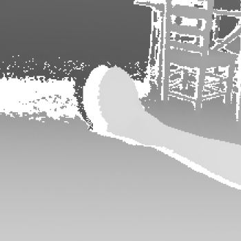
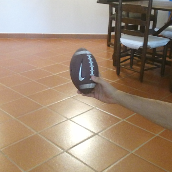
Fig. 3 Example of a depth map (dark is far) for the object 33 with a complex background. Chessboard pattern where the depth information is missing.
Finally, to make sure everything is there, you can check the exact number of (color + depth) images you're going to find for each object and session:
Object Detection
CORe50 can even be used for Object Detection. In this scenario, we have already provided Tensorflow records for setting up the training pipeline:
Given these 3 files, it is possible to set up a training pipeline according to the Tensorflow Object Detection APIs. Some visual results are shown in figure 4:
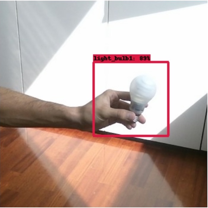
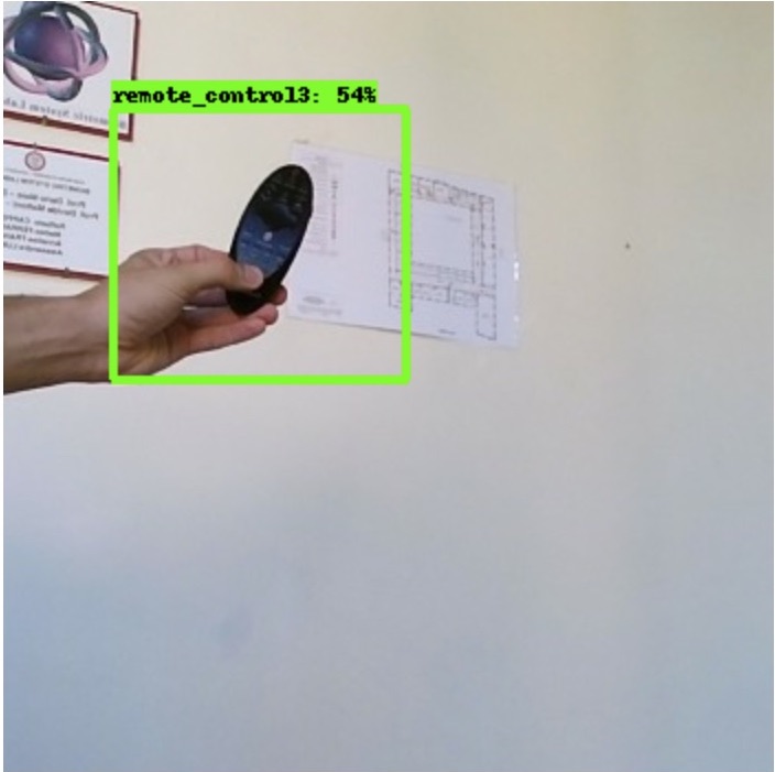
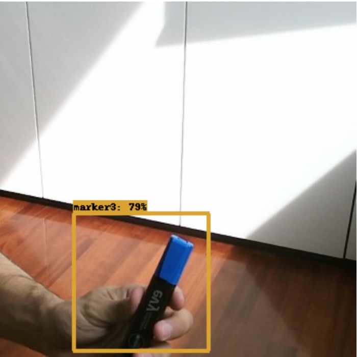
Fig. 4 Example of Object Detection using CORe50 as dataset.
However, if you wish to use another framework you can use comma separated files (.csv) that contain labels, id and bounding boxes for each image.
We tested object detection using a pre-trained SSD_MobileNet_v1 on COCO dataset and fine-tuning the last layers on CORe50. Performances stabilize around 20k and 30k iterations, with an accuracy up to 70% mAP. Further details are available on this repository.
We also make available an additional test set for detection in the clutter using the same objects used in the training set of CORe50 as well as additional out-of-sample objects of the same classes (see Fig. 5).
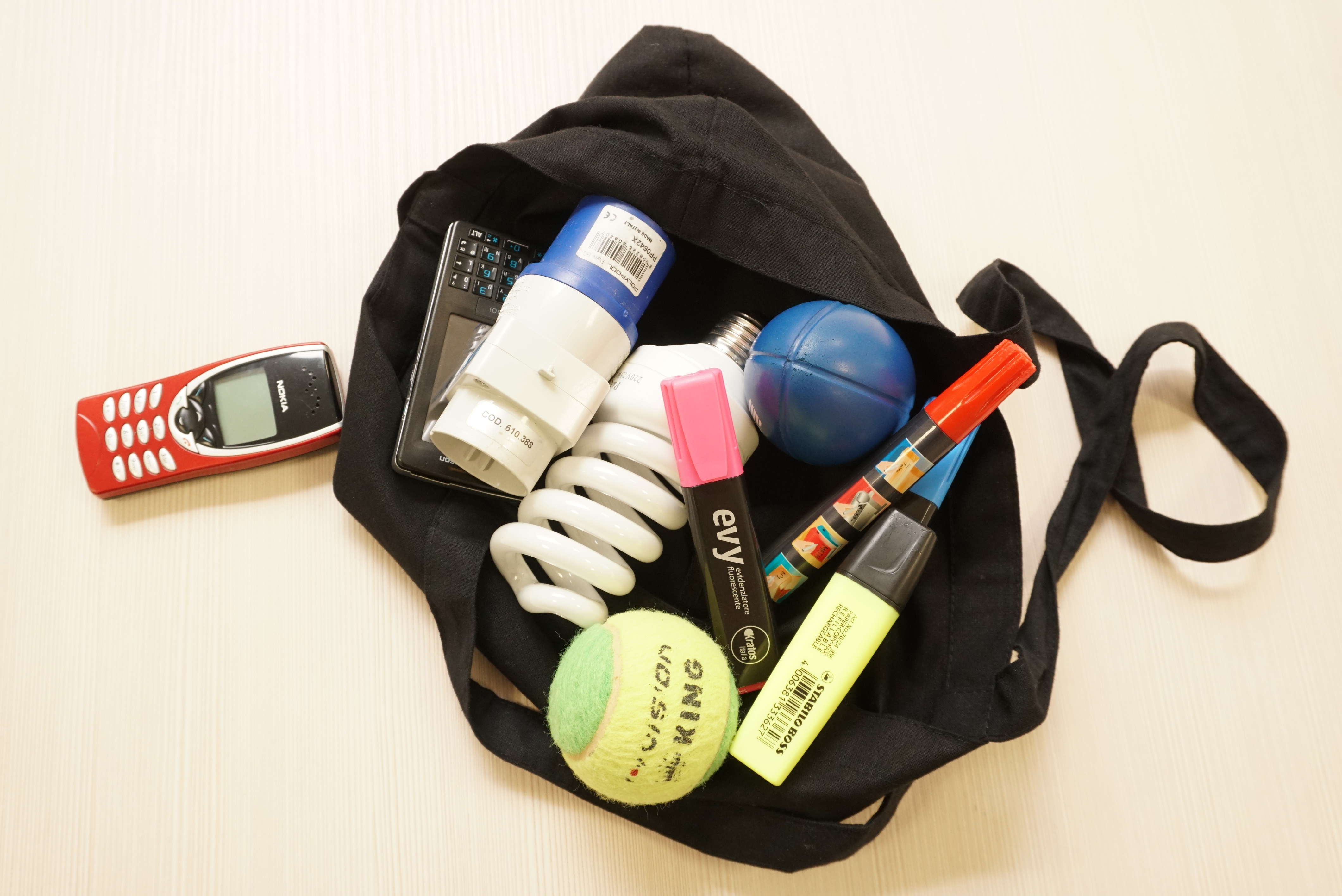
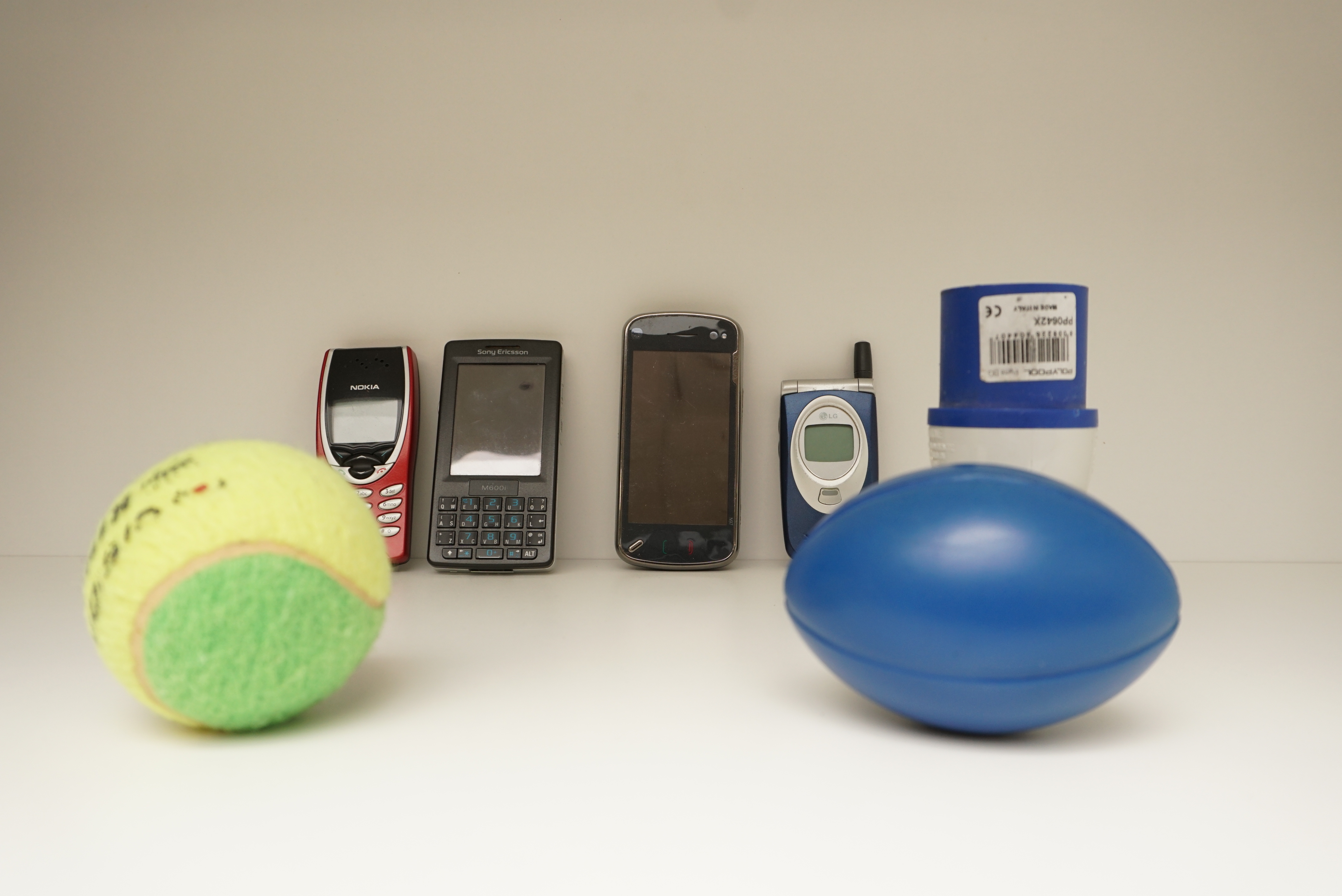
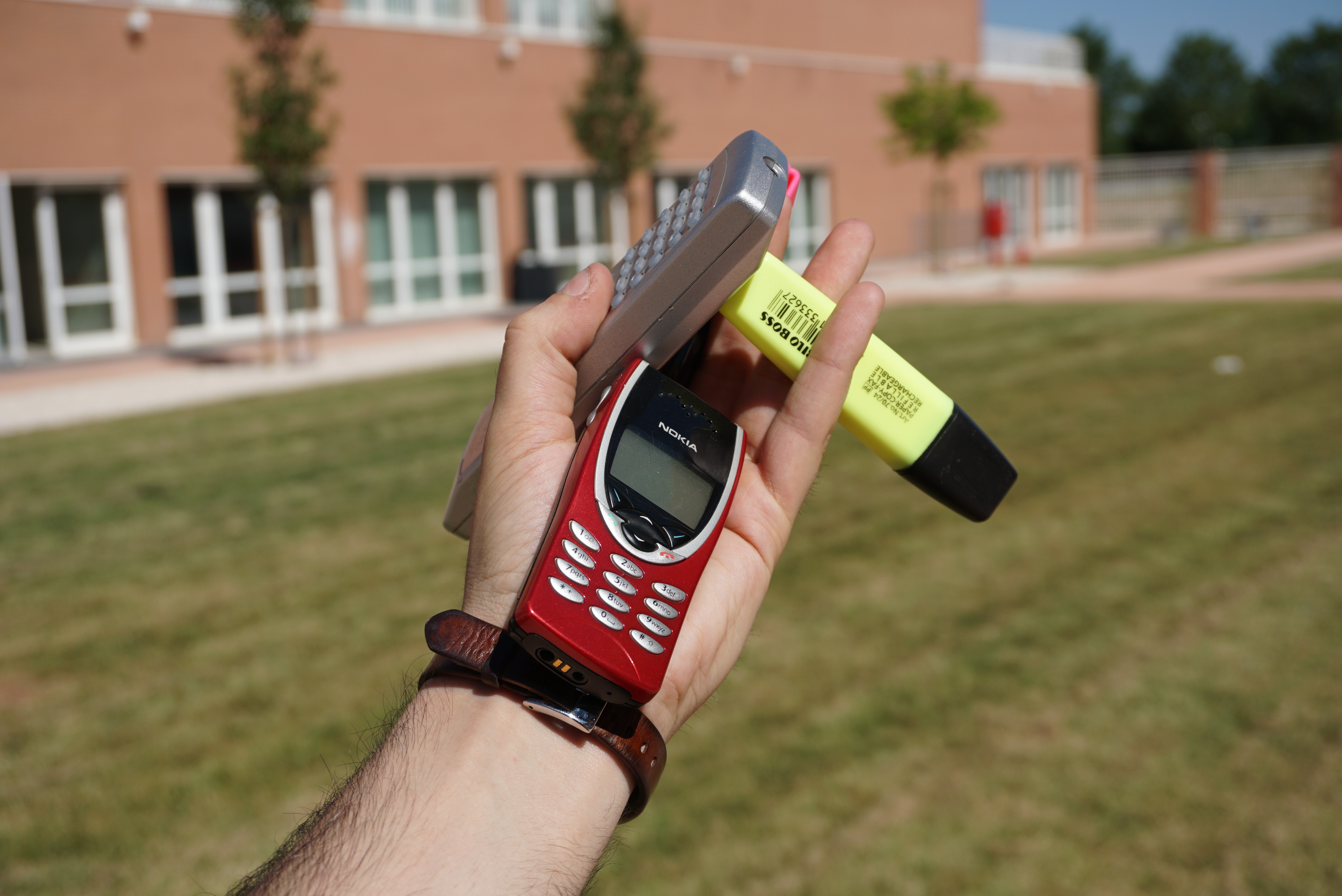
Fig. 5 Example of Object Detection in the Clutter.
Object Segmentation
It is possible to exploit depth information to approximately segment CORe50 objects. First, we created an algorithm that, given an image, discards all pixels belonging to the background. After that, we trained a SVM classifier to identify holding hand pixels. By deleting the background and the holding hand, what we got is the segmentation of the original object. These steps are shown in figure 6.
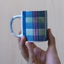
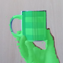
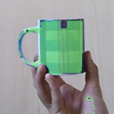
Fig. 6 Example of Object Segmentation on CORe50.
The code for object segmentation is available on this repository. Approximate object segmentation has already been shown successfull in many papers like "Learning Features by Watching Objects Move", 2016.
Configuration Files
Do you wanna use a different DL framework or programming language but still being able to compare your results with our benchmark? Well that's easy! Just download the batches filelists for each experiment in plain .txt format! The filelists directory tree will look like this:
filelists/
  |
  |--- NI_inc/
  |       |------ Run0/
  |       |         |------ train_batch_00_filelist.txt
  |       |         |------ train_batch_01_filelist.txt
  |       |         |------ ...
  |       |         |------ test_filelist.txt
  |       |
  |       |------ Run1/
  |       |------ ...
  |       |------ Run9/
  |
  |--- NI_cum/
  |--- NC_inc/
  |--- NC_cum/
  |--- NIC_inc/
  |--- NIC_cum/
PLEASE NOTE that:
- The order may highly impact the accuracy in a continual learning scenario! This is why a multiple runs configuration is needed;
- For the NC scenario the mappings "object -> label" are different for each run . That's because some CL strategies prefer labels to be continual for each incremental batch (i.e. if we have 3 objects we want the labels to be exactly 0, 1 and 2)!
 # loading the picked file
 >>> import pickle as pkl
 >>> pkl_file = open('labels2names.pkl', 'rb')
 >>> labels2names = pkl.load(pkl_file)

 # using the dict like labels2names[scenario][run]
 >>> print exps['ni'][0]
 {0: 'plug_adapter1', 1: 'plug_adapter2', ... }
Results
If you want to compare your strategy with our benchmark or just take a closer look at the tabular results, we are making available the tab separated values (.tsv) files for each experiment! Which you can easily import in excel or parse with your favourite programming language ;-) The format of the text files is the following:###################################
# scenario: NI
# net: mid-caffenet
# strategy: naive
###################################
RunID Batch0 Batch1 Batch2 Batch3 Batch4 Batch5 Batch6 Batch7
0 44,30% 35,50% 55,26% 55,86% 54,39% 48,90% 47,77% 60,71%
1 47,56% 48,94% 51,83% 53,64% 51,26% 43,39% 58,98% 55,61%
2 40,06% 53,04% 46,65% 45,19% 44,09% 50,92% 54,42% 57,01%
3 46,29% 48,66% 54,64% 52,48% 44,36% 51,55% 50,64% 44,26%
4 28,40% 43,77% 43,27% 51,00% 58,26% 56,89% 52,08% 61,94%
5 34,65% 34,36% 50,14% 56,89% 59,67% 56,66% 56,16% 52,66%
6 40,80% 51,92% 51,44% 53,12% 58,19% 49,72% 50,33% 48,14%
7 30,96% 51,54% 46,28% 51,69% 56,88% 55,44% 55,72% 49,98%
8 34,32% 32,19% 40,55% 52,06% 57,86% 57,41% 57,80% 61,86%
9 46,06% 47,62% 51,80% 46,92% 42,30% 57,70% 59,98% 50,01%
avg 38,59% 44,44% 48,90% 52,44% 53,88% 52,32% 53,77% 54,69%
dev.std 6,87% 7,88% 4,84% 3,59% 6,75% 4,74% 4,06% 6,18%
....
 # loading the picked file
 >>> import pickle as pkl
 >>> pkl_file = open('results.pkl', 'rb')
 >>> exps = pkl.load(pkl_file)

 # using the dict like exps[scenario][net][strategy][run][batch]
 >>> print exps['NI']['mid-caffenet']['naive']['avg'].values()
 [38.59, 44.44, 48.90, 52.44, 53.88, 52.32, 53.77, 54.69]
 >>> print exps['NI']['mid-caffenet']['naive']['avg']['Batch0']
 38.59
Code and Data Loaders
The Python code for reproducing the experiments in the paper is already available in the master branch of this github repository!As you might have noticed, assessing your own CL strategies on CORe50 wouldn't be as simple as loading the npz file since you have to deal with a number of runs and configurations. That's way we also provide a super fast and flexible Python Data Loader which can handle that for you. For example:
 # importing CORe50
 >>> import data_loader
 >>> train_set = data_loader.CORE50(root='/home/admin/core50_128x128', cumul=False, run=0)

 # Using the data loader
 >>> for batch in train_set:
 ...     # This is the training batch not the mini-batch
 ...     x, y =  batch
Take a look at the Python class here for more details. As you can see we thought at two modalities. The first one for small RAM devices where we load the batch imgs on-the-fly as they are needed and the second one in which we preload the entire dataset and we use a Look-UP table to figure out which subset of data we need.
if you are a PyTorch user, we have just implemented the Pytorch Data Loader (pending Pull Request), you can download here but up to now it has only the "loading on-the-fly" (even if multi-threads) modality.
If you want to contribute or you find a bug, please make a PR or simply open an issue (also questions are welcomed)! We guarantee at least an answer in 48hrs! :-)
Contacts
This Dataset and Benchmark has been developed at the University of Bologna with the effort of different people:- Vincenzo Lomonaco • PhD Student
- Davide Maltoni • Professor
- Riccardo Monica • Master Student
- Martin Cimmino • Master Student
- Giacomo Bartoli • Master Student
For further inquiries you are free to contact Vincenzo Lomonaco through his email: vincenzo.lomonaco@unibo.it